TagLab Documentation

• Interface
• Create and manage projects
• Import options
• Export options
• Tools
• Labels operations
• How-to
  • Learning pipeline
  • Digital elevation models
  • Multi-temporal comparison

Interface

The toolbar is located on the left side of the interface; it contains the following operation buttons, individually activable:

• Move Enables Pan/Zoom operations.
• 4-clicks segmentation AI assisted tool for the interactive boundaries tracing using the four extremes.
• Positive/negative clicks segmentation AI assisted tool for the interactive boundaries tracing using inner and outern points.
• Freehand segmentation Pixel-based drawing tool.
• Assign class Tool for the class assignment (select + A).
• Edit border Quick contour editing tool.
• Cut segmentation Draws curves to quickly separate labels.
• Create crack Interactively creates inner cracks.
• Measure tool Takes linear measures, between a pair of points or objects centroids.
• Fully automatic classification Allows to select a pre-trained semantic segmentation network from the ones available, and apply it new data.
• Split screen Splits the working view in two sincronized views.
• Compute automatic matches Computes automatic correspondences between semantically segmented regions displaying them on a table.
• Add manual matches Allows the manual editing of correspondences.

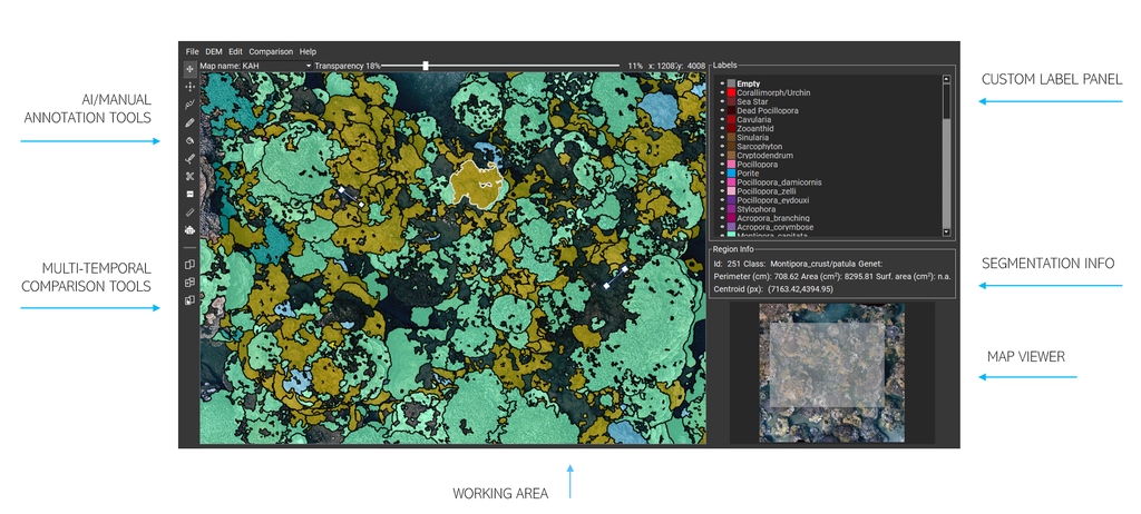
The Working View displays the image data to annotate. Navigation is straightforward: zoom (wheel to zoom in and out) is always allowed, panning is enabled only when the Move tool is active or by pressing the Ctrl+ mouse left button (when one of the other tools is active). Above the Working View, a slider allows adjusting segmentations transparency.

On the right side, the Labels Panel contains your custom list of colours and class names; you can configure labels by editing the dictionary available in the .config file in your TagLab folder. The Eye icon controls the visibility of each class which be switched singularly or in groups (by pressing Ctrl or Shift). This helps to visualize the distribution of specific species and, considering that only visible tags are processed, the export of targeted maps, tabs, or statistics.

The Region Info box shows properties related to the selected object as id, genet, coordinates, class, perimeter, area, and surface area. This information is updated by double-clicking the object.

The Map Viewer, on the bottom right of the interface, highlights the map region under viewing in the Working View, assisting the navigation of extensive maps. The Map Viewer is interactive, too; the working area can be selected by a single click or by panning on the rectangle of interest.

Create and manage a project

File > Add New Map

Choose a name and browse data from your PC. Be careful:

• TagLab only supports .jpg and .png RGB images with a maximum size of 32767x32767 pixels.
• TagLab doesn't support images having a transparency channel.
• The loading of a .tiff file with the DEM is not mandatory.

Please, fill all the fields in the Map Settings menu. TagLab will use the Acquisition Date for the multi-temporal comparison, the Pixel Size to convert pixels regions in cm² and lengths in cm. By clicking apply, you create a new TagLab map. If TagLab crashes after the data loading, the image format is probably not supported. In TagLab, a map is a data layer containing the ortho, the DEM (if existing), related info and your region-based annotations. TagLab supports the creation of multiple maps for multi-temporal comparison. You can select visualized maps through the Map Name field on the top of the Working View.

File > Edit Map Info

You can edit the Map Setting fields of all your TagLab maps in a further moment by using the Edit Map Info. However, you are not allowed to change the ortho.

File > Save Project

It saves the current project. The project file contains one or a set of TagLab maps. References to the loaded map, the settings, and to annotations (as a list of coordinates and assigned classes) are saved in a JSON file.

File > Open Project

It allows loading an existing project. If the image data has been moved into another folder, Taglab asks you to re-locate and load them again. The project file can be moved anywhere. Recents open projects are directly visible in the File menu.

Import options

File > Import Options> Import Label Image.

This option allows you to poligonize a co-registered label image and load the polygons as annotations superimposed on your ortho. The label image must have a black RGB(0,0,0) background, and the foreground classes must be present in your .config file. It may be useful to use Taglab edit tools on a previous segmentation.

File > Import Options> Add Another Project.

Append a project (one or a set of TagLab maps) to the current one.

Export Options

File > Export Options > Annotation as Data Table

Saves a .csv file containg a unique id, genet, class information, area, perimeter, centroids coordinates for each polygon.

File > Export Options > Annotations as Label Image

Saves a .png pixel-wise segmented image with a black background and colored foreground classes according to the visible classes in your label panel. Class visibility might be switch on and off using the Eye icon.

File > Export Options > Export Annotations as a GeoTiff

Exports a geo-referenced labelled image.

File > Export Options > Annotations as Shapefile

Exports visible annotations as a geo-referenced shapefile.

File > Export Options > Histogram

Creates a histogram containing all the foreground classes checked in the menu. It automatically display per-class coverage.

File > Export Options > Training Dataset

Export squared tiles of 1026 pixels with an overlap of 50%. TagLab exports each RGB map tile and the corresponding label with the same suffix. For more information, please refers to Learning pipeline.

Commands

Undo and Redo operations work with Ctrl + z, Crtl + Shift + z

Select

Operations can only be applied on selected labels. For the single label selection, double click inside a label; the polygon outline changes from black to white. Almost all operations work with a single selected label, except delete, boolean operations (merge, divide, subtract), assign class, that allows multiple selections. Labels can be added to the selection using Shift + left click. A group of label can be selected by dragging a rectangular window (Shift + left click + drag). To select labels by window dragging, be sure to include them entirely in the rectangle.

Confirm operation

To carry out an operation, select a tool, select a polygon if required by the process, perform edits, and then press Space bar to apply it.

Reset tool

Any operation can be canceled by pressing Esc before confirmation.

Tools

The zoom is always active; all tools are activable singularly. In most tools, the tracing/editing actions must be confirmed by pressing the Space bar.

Move

When the move tool is selected, the image pan operation is active (left click + drag). When one of the other tools is selected, the pan operation is allowed only by pressing Ctrl +left click + drag.Pan and zoom operations in the Working Area are synchronized to the Map viewer. The Map Viewer is interactive too; you can use it to navigate large ortho, your current position is highlighted.

Assign

When the assing (buket icon) tool is active, all the clicked polygons assumes the class name and the correspondig color values of the selected class in the labels panel. Multiple selection is allowed by pressing Shift (same options as below). If multiple polygons are selected and the bucket tool is active, all blobs are simultanously assigned to the same class.

Freehand segmentation

When the Freehand segmentation is active, users can draw a pixel-wise curve of a fixed thickness of 1px. The curve doesn't need to be drawn continuously but can be drawn in different overlapping segments. The operation is applied by pressing Space bar, and the curve/curves became a polygon. Only closed curves can become polygons; unclosed curves are automatically removed. Curves might intersect themselves several times, but they always produced a unique closed polygon without holes. There is no need to match the start and the end of the line exactly. Additional segments, inside or outside the polygon, are automatically removed too. The operation can be discarded at every moment (before confirming) by pressing Esc. Drawing is always allowed also internally to another blob.

Edit border

When this tool is selected, the user can arbitrary draw curves on a single selected polygon. Areas included or excluded from the edit curves are automatically added or removed from the selected polygon. Information in the info panel is automatically updated. If no polygon is selected or multiple polygons are selected, the edit operation cannot be applied; select a single area and press Spacebar again.

Curves don't need to continue and can be concave or convex. Curves must cross the polygon outline at least twiceto be effective; otherwise, they will automatically remove them. You can edit any inner contours following the same criterion. The snapping option is always active, and the resulting polygon is cleaned from unwanted scratches.By pressing Esc before confirming, the tool will remove all the editing curves. Undo and Redo operations are always allowed. Drawing a closed editing curve inside a polygon creates holes.

Cut segmentation

This tool works exactly like the Edit border tool except that the regions subtended by the edit curves are not removed but separated from the current polygon. After confirmation (Space bar) of the cut operation, they become different segmented regions. The class assigned by default is the same as the starting segmentation.

Create crack

The Create crack tool is useful to create empty cracks inside a polygon quickly. When the tool is active, clicking on a point inside a crack opens the Crack window. The window has a slider that allows adjusting the selected area. The result of the selection is visible through the preview (which is zoomable). The operation is confirmed by pressing the Apply button..

Measure tool

The Measure tool can measure the distance (express in cm if the pixel size is known) between two points or the distance between polygons' centroids. In this last case, the user has to select two polygons, and the tool will snap the measure to the centroids.

4-clicks segmentation

This tool implements a CNN for the interactive tracing of object boundaries. The user, helped by the cross cursor, places four points at the object's extremes (extreme top, extreme bottom, extreme left, extreme right). There is no need to follow a specific order, but it's necessary to position them as accurately as possible near the extremes. After placing the fourth point, the contours of the object are automatically delimited through a neural network called Deep Extreme Cut. This tool works only if you have the network's weights properly placed in TagLab's models folder.

Positive/negative clicks segmentation

This tool implements a CNN for the interactive tracing of object boundaries. To use this tool efficiently, the user must zoom in on the object to be segmented, framing it completely, pressing the Shift, picking positive clicks inside the object (green color), and negative external clicks (red color). The segmented area is visualized progressively; to create a polygon and confirm the operation, press Space bar. Be sure to frame entirely but strictly the object, as the CNN behind works on the entire area framed by the Working Area. You can use this tool with the same procedure for the click-based correction of already existing polygons. In that case, select the polygon and frame the portion to be corrected. The tool implements the neural network Reviving Iterative Training with Mask Guidance for Interactive Segmentation , optimized for working on complex shapes. This tool works only if you have the network's weights properly placed in TagLab's models folder.

Fully automatic segmentation

This tool classify pixels using an optimization of the fully automatic semantic segmentation network DeepLab V3+ . For a detailed explaination about its usage, please refers to Create custom classifier.

Labels Operations

Assign

A This shortcut assigns the selected class to the selected polygon/polygons.

Fill

F By pressing F with a selected polygon, inner holes are filled.

Delete

A Canc Remove selected polygon/polygons.

Merge

M This tool creates a single polygon from selected overlapping polygons.

Divide

A D This tool separate two overlapping polygons creating a two non-overlapping boundaries according two the selection order. The contour of the first prevails over the second.

Subtract

S This takes two selected polygons and remove the second from the first according to the selection order. When the second blob lies inside the first, it creates a hole.

Refine

R By pressing R on a selected polygon, the tool will adjust contours according to the image gradient. The Refine tool implements a variant of the Graph-Cut algorithm to significantly improve the objects' contours accuracy without straying too far from the existing ones.

How To

• Learning pipeline
• Digital elevation models
• Multi-temporal comparison

Learning pipeline

TagLab supports you in creating automatic classifiers optimized on your labelled data, automating your annotation and analysis pipeline. Custom models can be saved and later used to classify new data (using the Fully automatic segmentation tool).

How to export a training dataset

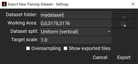
From the File > Export > Export New Training Dataset opens the following window:

Export Dataset Settings

During the export, orthos are cropped into tiles (small sub-images) matching the network input size and partitioned into training, validation tiles, and test tiles. In deep learning, training tiles are used in network weights optimization (actual learning), validation tiles to select the most performing network (weights combination), and the test tiles to evaluate the new classifier's performance. The majority of the tiles, about 75%, are dedicated to learning, 15% to validation and the remaining 15% to testing. This introduction helps you to understand the exporting settings (see figure below).

Please note, each different label colour is considered as a different class; if you need to exclude some classes from the training, you need to export the dataset disabling the class's visibility using the eye icon.

Dataset folder: folder where you will save the dataset; training, validation, and test tiles are stored in sub-folders.

Working area: part of the orthoimage used to create the dataset (visualized with a purple dashed rectangle). By default, the working area is the entire orthoimage, but you can frame a portion by clicking the button on the right and drawing a rectangle on the orthoimage. Be sure to include in the working area only totally labelled data, avoiding non labelled objects belonging to some minority classes.

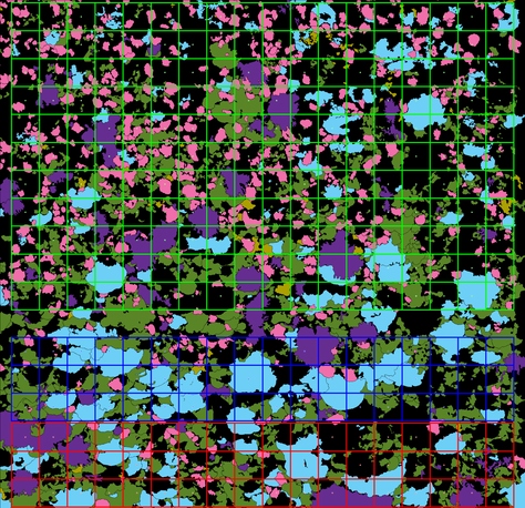
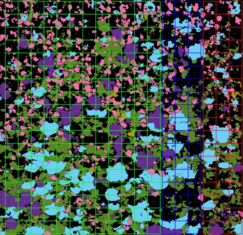
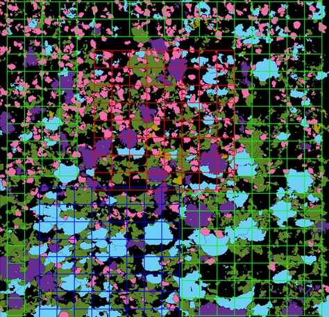
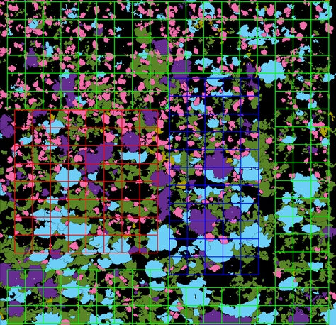
Dataset split: Training, validation, and test tiles are extracted by subdividing the working area; they represent 75%, 15%, and 15% of the ortho, respectively. The partition can be Uniform vertical (from top to bottom), Uniform horizontal (from left two right), Random (randomly sampled areas), or Ecological-inspired. This last option has been designed for researchers working in marine ecology. Training, validation, and test areas are chosen according to some landscape ecological metrics scores, so they are all equally representative of the species distribution. Regardless of the partition, tiles are generated by clipping the sub-areas in scan order. The figure below shows the sub-area partition and clipped tiles, according to the different Dataset Split options.

Target scale: orthos and labels are rescaled to a common scale factor before the tiles export. This is useful to create a dataset from a set of ortho mosaics having severe differences in pixel size. If you want to create a dataset from more than one annotated ortho, you have to export tiles in the same folder; the scale factor helps you choose an average pixel size and uniform your data.

Oversampling: when this option is checked, the export tries to balance the classes by sampling a higher number of tiles from rare objects.

Show exported tiles: save in the Taglab’s directory an image called tiles.png showing the scheme (figure below) of exported tiles.

How to train your network

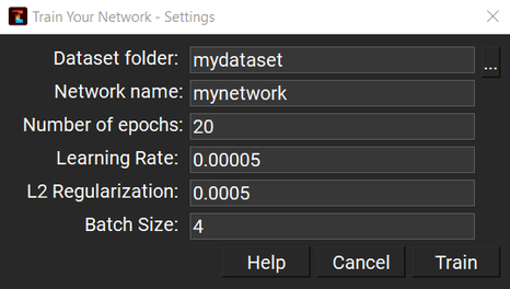
When the dataset is ready, you can create your custom classifier from File > Train Your Network . This feature creates the new classifier by optimizing a DeepLab V3+ on your data.

Train Your Network Settings

Dataset folder:

indicate your dataset’s folder.

Network name:

choose a name for the new classifier.

Number of epochs:

a typical number is between 50 and 80; the higher this value, the longer the time required for training.

Learning rate:

this parameter should be changed only if you have some machine learning knowledge. The default value is chosen to work well in many different application cases.

L2 regularization:

this parameter should be changed only if you have some machine learning knowledge. The default value is chosen to work well in many different application cases.

Batch size:

higher is better; 4 is a reasonable choice. A number greater than 8 can cause memory issues even if you have a GPU with 8 GB of RAM.

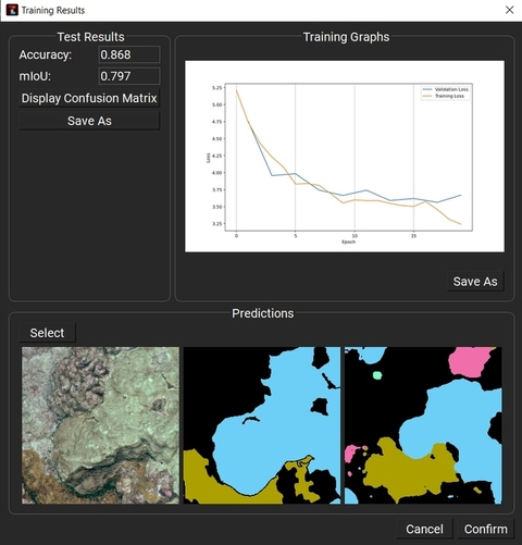
At the end of the training, TagLab will display training metrics and graphs in the Training Results window. Indicatively, the more the accuracy and mIoU values get closer to 1, the higher is the quality of your classifier (values of mIoU around 0.8 can be considered good). To check the classification correctness, you can select a tile from the test dataset and see how the model has classified the pixels in the Prediction window. By confirming, the classifier is saved in the TagLab's models folder; it can be loaded using the Fully automatic segmentation tool.

Training Result Window

Pratical hints

• Larger training dataset outputs automatic models with better performance.
• A training session with a lot of data and a lot of epochs may need several hours.

Fully automatic segmentation

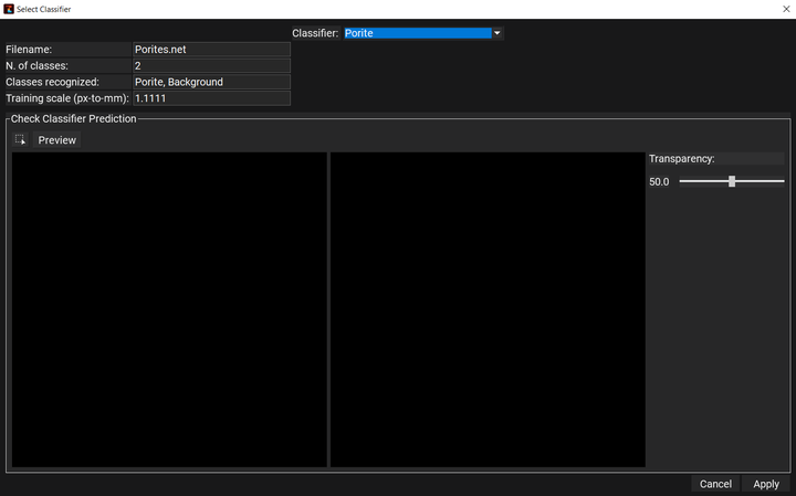
The Fully automatic segmentation tool allows you to select a classifier between the available ones and infer the semantic segmentation on a new ortho. Activating the tool opens the Select Classifier window, where the classifier can be selected through the combobox Classifier.

Information like the number and the name of recognized classes (a.k.a number of colours in your training dataset) and the training scale factor are reported immediately below. The new ortho is rescaled at the training scale before the classification.

Before launching the classifier on the entire map, you can select a region of the ortho mosaic by clicking the button and previewing the classification on the selected region by pressing the Preview button. The button Apply launches the automatic classification on the entire ortho mosaics; the progress bar illustrates the classification process's progress. During the classification, TagLab creates a temp folder in the TagLab directory containing all the classified tiles and an image, called labelmap.png, the average aggregation of all the scores on the entire ortho.

WARNING! When the automatic classification finishes, TagLab asks to save the project and re-open the tool. If you don’t save the project, you can re-open it and load the labelmap.png image from File > Import Label Image.

Digital elevation model (DEM)

Switch between RGB/DEM

If you have loaded a Digital elevation model (DEM), you can switch between the ortho and the DEM by pressing the key C or clicking on the corresponding voice from the DEM menu.

Compute surface area using DEM information

DEM can be used to compute an approximation of each segmented region's surface area. This measure gives a better quantification of change between objects than the planar area.

The surface area is computed only on the ortho currently displayed on the Working Area. So, if your project contains more than one ortho, you need to launch the surface area computation for each one.

Clipping a DEM

The menu option DEM > Export Clipped Raster allows clipping a DEM using the segmented regions. The result, a geo-referenced raster object (.tiff file) containing only the depth information of the segmented regions, can be imported in GIS software to perform further DEM processing operations (such as the surface rugosity calculation of a specific class).

Multi-temporal comparison

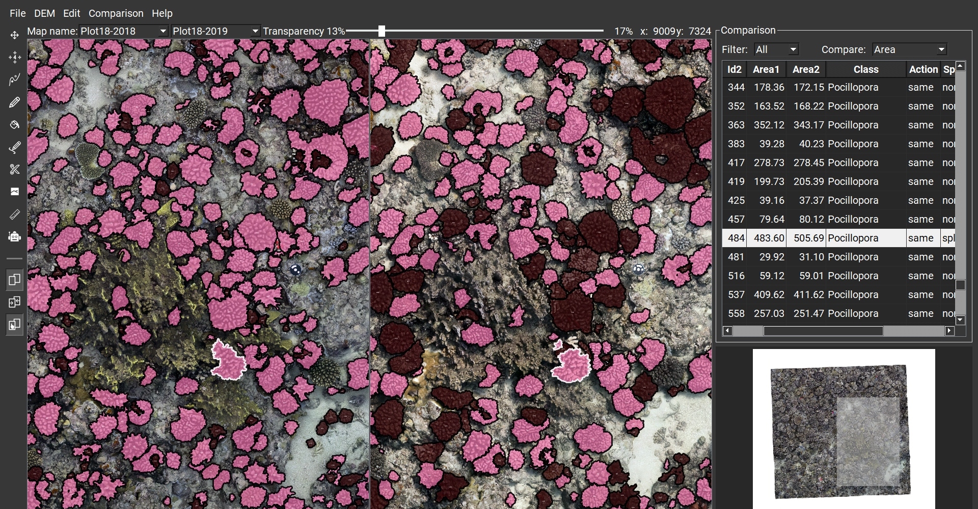
TagLab allows loading co-registered orthos, reconstructed from temporally different surveys, and tracks the segmentations morphological changes. To facilitate the visual comparison, by clicking the Split screen button, maps (orthos and labels) are navigated through synchronized paired views. You can compare plots only in pairs; when your projects contain more than two labelled orthos, you can select the ones to compare using the Map Name menu on the top.